Your paper, your format
A two-host conversation, a focused walkthrough, or the quick essentials, in the voice you choose.
PaperCast
Each week, the most consequential papers in seven disciplines, narrated in your choice of three formats. Skim the transcript, jump to what interests you, and trace every claim back to the source.
Listen below for this week's free episode. Join the waitlist to unlock the full seven-discipline catalog.
Loading transcript…
The free preview plays one paper end-to-end. Join the waitlist to unlock the full peer-reviewed catalog, switch papers, and adjust persona, style, and voice.
A two-host conversation, a focused walkthrough, or the quick essentials, in the voice you choose.
Tap any line in the transcript to jump to exactly where it lives in the source. Trust is verifiable, not asked for.
One consequential paper per field, each labeled by version, peer-reviewed, preprint, or manuscript, so you know what you're hearing.
Every episode is backed by the full rendered paper. Switch from the audio to the text whenever you want to go deeper.
Debrief
Type what you are researching. Debrief finds papers by meaning across every discipline, opens the top result, and answers your questions with citations to the exact section and page.
With the increasing demand for battery energy density and safety, solid-state batteries are expected to become one of the ideal energy storage devices. Aiming at compensating for the research lack of modeling and state estimation of solid-state batteries, this paper proposes a state of charge (SOC) estimation method based on the electrochemical impedance spectra (EIS) of sample solid-state batteries that consider both accuracy and speed. The SOC estimation model is established using Gaussian process regression by extracting the low- and medium-frequency semicircular parameters that vary markedly with SOC. Considering the online application of the method, the fixed-frequency test impedance is selected as the characteristic parameter to achieve the SOC estimation that takes both accuracy and speed into account, and the method is still applicable under different state of health (SOH). Considering the existence of 3 impedance spectral semicircles in this solid-state battery, the RQ (parallel connection of resistors and constant phase element) process is added to establish a fractional-order model and the fractional-order extended Kalman filter (FOEKF) algorithm is developed. What is more, the FOEKF algorithm and SOC-OCV curve are constructed as a control group to analyze the accuracy, advantages, and disadvantages of the proposed SOC estimation method. The results show that the unique EIS performance of this solid-state battery is more conducive to achieving the estimation of the battery SOC. The application of the EIS online implementation method is expected to rely on the fixed-frequency test to achieve online accurate estimation of the SOC of solid-state batteries.
Is this the paper you were looking for?
This paper proposes a state of charge (SOC) estimation method based on the electrochemical impedance spectra (EIS) of sample solid-state batteries, aiming to balance accuracy and speed S1, p.1.
The contributions include:
The results indicate that the unique EIS performance of the solid-state battery is favorable for achieving the estimation of the battery SOC S1, p.1. Furthermore, the estimation model based on EIS characteristic parameters allows for fast and accurate SOC estimation, particularly when considering online implementation using fixed-frequency testing below 2 Hz Introduction, p.2. The method also proves applicable under various SOH conditions Introduction, p.2.
The paper utilizes several methods, models, and experiments:
The paper reports several findings regarding the model's ability to fit the EIS of the solid-state battery, stating that the model can better fit the EIS of the solid-state battery S18, p.9. Furthermore, the results demonstrate that the estimation model based on EIS characteristic parameters allows for fast and accurate SOC estimation, particularly when considering online implementation using fixed-frequency testing below 2 Hz Introduction, p.2. The method also proves to be applicable under various SOH conditions Introduction, p.2. The convergence speed and estimation accuracy of the FOEKF algorithm were verified by setting different initial SOC values, such as 0%, 30%, 60%, and 90% under FUDS conditions S20, p.13 S20, p.13.
The research gap motivating this paper is that while research on modeling and parameter estimation for lithium-ion batteries is relatively mature, the study of emerging solid-state batteries is still in its early stages, and research concerning performance and parameter estimation for solid-state batteries is lacking Introduction, p.2. Specifically, there is a lack of research on the utilization performance and parameter estimation of solid-state batteries Introduction, p.2. Another stated gap is the lack of modeling and state estimation for solid-state batteries S1, p.1.
The paper utilizes several experimental methods, models, and algorithms:
Experimental Methods:
Models:
Algorithms and Estimation Methods:
This paper aims to address the gap in research concerning solid-state batteries by analyzing the third semicircle trend of the EIS in relation to the battery's State of Charge (SOC) Introduction, p.2. The novel approach involves extracting impedance parameters at various frequencies using EIS testing to develop a SOC estimation model for solid-state batteries Conclusion, p.15. This model allows for fast and precise SOC estimation for solid-state batteries Conclusion, p.15.
A Novel State of Charge Estimation Method Based on Electrochemical Impedance Spectroscopy for Solid-State Batteries of Next-Generation Space Power Sources under Different States of Health
Citation: Sun B, Pang J, Zhu L, Zhao X, Zhang W, Ma S, Liu X. A Novel State of Charge Estimation Method Based on Electrochemical Impedance Spectroscopy for Solid- State Batteries of Next-Generation Space Power Sources under Different States of Health. Space Sci. Technol. 2025;5:Article 0198. https://doi. org/10.34133/space.0198
Bingxiang Sun¹,²*, Junfeng Pang¹,², Liying Zhu³, Xinze Zhao¹,²*, Weige Zhang¹,², Shichang Ma¹,², and Xiaopeng Liu¹,²
National Active Distribution Network Technology Research Center (NANTEC), Beijing Jiaotong University, Beijing 100044, China. Key Laboratory of Vehicular Multi-Energy Drive Systems (VMEDS), Ministry of Education, Beijing Jiaotong University, Beijing 100044, China. Beijing Institute of Spacecraft System Engineering, Beijing 100094, China.
Submitted 22 January 2024 Revised 30 May 2024 Accepted 14 July 2024 Published 29 April 2025
Copyright © 2025 Bingxiang Sun et al. Exclusive licensee Beijing Institute of Technology Press. No claim to original U.S. Government Works. Distributed under a Creative Commons Attribution License (CC BY 4.0).
*Address correspondence to: bxsun@bjtu.edu.cn (B.S.), 21117037@bjtu.edu.cn (X.Z.)
With the increasing demand for battery energy density and safety, solid-state batteries are expected to become one of the ideal energy storage devices. Aiming at compensating for the research lack of modeling and state estimation of solid-state batteries, this paper proposes a state of charge (SOC) estimation method based on the electrochemical impedance spectra (EIS) of sample solid-state batteries that consider both accuracy and speed. The SOC estimation model is established using Gaussian process regression by extracting the low- and medium-frequency semicircular parameters that vary markedly with SOC. Considering the online application of the method, the fixed-frequency test impedance is selected as the characteristic parameter to achieve the SOC estimation that takes both accuracy and speed into account, and the method is still applicable under different state of health (SOH). Considering the existence of 3 impedance spectral semicircles in this solid-state battery, the RQ (parallel connection of resistors and constant phase element) process is added to establish a fractional-order model and the fractional-order extended Kalman filter (FOEKF) algorithm is developed. What is more, the FOEKF algorithm and SOC-OCV curve are constructed as a control group to analyze the accuracy, advantages, and disadvantages of the proposed SOC estimation method. The results show that the unique EIS performance of this solid-state battery is more conducive to achieving the estimation of the battery SOC. The application of the EIS online implementation method is expected to rely on the fixed-frequency test to achieve online accurate estimation of the SOC of solid-state batteries.
With the continuous promotion of the “double-carbon” strategy, energy storage technology is poised for broad application prospects. Lithium-ion batteries have gained widespread use in electronic products and power energy storage, owing to their high capacity density, high power density, lack of memory effect, low self-discharge rate, and long service life [1,2]. However, the energy density of the existing material system in lithium-ion batteries has reached its limit. With the rapid progress of new energy technologies and the increasing number of power battery applications in new energy transport vehicles, higher demands are being placed on energy density, safety, and battery volume weight [3]. In contrast to conventional lithium-ion batteries, solid-state batteries utilize solid electrodes and solid electrolytes, eliminating the need for flammable and explosive liquid
electrolytes. They offer higher energy density and lower power density, making solid-state batteries much lighter than lithium-ion batteries of the same capacity. As a result, solid-state batteries are considered a promising alternative energy source for electric vehicles and energy storage systems, given their safety and energy density advantages [4–7]. According to South Korean market research firm SNE Research, the market space for solid-state batteries is expected to reach 20 billion Chinese yuan in 2030, surpassing lithium-ion batteries as the mainstream choice for electric vehicle batteries [8]. However, solid-state batteries differ substantially from conventional lithium-ion batteries in their material system. This leads to fundamental changes in physical, chemical, and mechanical processes, such as material transport, interface electrochemistry, and stress evolution within the battery [3]. Therefore, a systematic analysis of the similarities and differences between solid-state batteries and lithium-ion batteries is essential. This analysis should encompass aspects like characterization technology and theoretical mechanisms to comprehensively strengthen the research theory of solid-state batteries and drive their large-scale market applications.
In recent years, the research on solid-state batteries is still in the stage of material research and improvement. Most of the reviews on solid-state batteries also focus on solid-state electrolytes with high ionic conductivity, electrochemical stability, and mechanical properties, as well as structural and interfacial improvement strategies for composite electrodes [9–13]. There are also some literature on the development and research outlook of solid-state batteries [14–16], but the research on the utilization performance and parameter estimation of solid-state batteries has hardly appeared. Currently, there is only one patent in the public information that mentions SOC estimation for solid-state batteries, which is performed by extracting battery voltage, current, temperature, and power as feature parameters. The validation values are output by 3 models and fused with the original features, and the gradient boosting decision tree model is selected for SOC prediction [17]. Therefore, in this paper, we test the solid-state battery from a lithium-ion battery and try to establish the model and parameter estimation method applicable to solid-state batteries.
Equivalent circuit models are divided into integer-order and fractional-order models according to the composition of circuit elements. The integer order model does not consider the internal reaction mechanism of the battery and mainly reacts to the external characteristics of the battery with fewer parameters, which makes it easy to derive the system space equation of state. It is widely used in system simulation and real-time control, and also has a wide range of applications in battery-related systems. The fractional-order model replaces capacitance C with constant phase element (CPE; commonly used Q) and introduces a fractional-order operator, which has a memory effect and is suitable for describing a memory hysteresis system. For example, modeling with electrochemical impedance spectroscopy (EIS) as a data source is often fitted with a fractional-order model. Hu et al. [18] carried out the establishment and parameter identification of a fractional-order model based on a hybrid multi-particle swarm algorithm, and used a second-order RQ model to verify the dynamic working conditions. Sun et al. [19] carried out a study of a variable-order fractional-order model based on the electrochemical impedance spectra of lithium-ion batteries and verified the model’s good accuracy with parameter identification via the FORPRLS algorithm. Fractional-order models with 1 or 2 RQs were used to estimate the SOC, and better results than the same RC (parallel connection of resistors and capacitance) model were achieved [18,20].
The most widely used method for estimating the state of charge (SOC) of a battery is the ampere-time integration method. Currently, most of the battery management systems (BMSs) also use the ampere-time integration method to estimate the SOC of the battery, which does not require modeling, is simple to implement, and is easy to operate. However, the method relies on the accurate acquisition of the initial value, and if the error of the initial value is large, the estimation results become inaccurate and cannot be corrected. At the same time, the accuracy of current acquisition also greatly affects the accuracy of estimation. SOC estimation based on the extended Kalman filter (EKF) algorithm is to expand the battery state-space equations using the Taylor series, and considering the computational complexity, the first order is mostly retained to linearize the nonlinear system. Reshma and Manohar [21] achieved the estimation of battery SOC by a dual adaptive Kalman filtering algorithm based on a first-order RC equivalent circuit using an improved remora optimization algorithm. Zhao et al. [22] also used a fuzzy method-based adaptive Kalman filtering based on an equivalent circuit, which improves the accuracy of the first hundreds of SOC estimation. Xiong et al. [23] used a fractional-order traceless Kalman filter (KF) to estimate SOC, which proves that the method is capable of achieving accurate estimation of battery terminal voltage and SOC under battery operating conditions over a wide range of temperatures and aging levels. Mawonou et al. [24] establishes a fractional-order model based on the EIS and estimates SOC based on the EKF, which provides a higher level of accuracy compared to the classical equivalent circuit. In addition to algorithm-based SOC estimation, Rodrigues et al. [25] and Buller et al. [26] investigated the variation rule of EIS with SOC for lithium cobalt acid batteries, and the semicircular diameter of the mid-frequency region of EIS monotonically decreases with the increase of SOC. This provides a new method for the estimation of battery SOC.
With the in-depth research on EIS, more and more online methods for obtaining impedance spectra have been published. Zhu et al. [27] used a BMS to generate excitation signals to obtain the battery impedance at different frequencies, realizing the online application of impedance spectra. Su et al. [28] achieved the online acquisition of impedance spectra in the low-frequency band below 2 Hz by injecting a stepped wave instead of sinusoidal waveforms. Sihvo et al. [29] used PRBS (pseudo-random binary sequence) as a reference for the current of discharged batteries and applied the discrete Fourier transform to the measurement of the impedance frequency response to achieve online measurement of lithium-ion battery impedance. Lyu et al. [30] achieved a fast measurement of impedance in the frequency range of 1 kHz to 0.01 Hz based on a hardware circuit by generating a sinusoidal excitation signal from an upper computer and performing a fast Fourier transform of the battery voltage response. Therefore, with the deepening of the research, the online acquisition of impedance spectra is no longer a difficult problem, and the engineering application of impedance spectra becomes possible.
Up until now, research on modeling and parameter estimation of lithium-ion batteries has reached a relatively mature stage with numerous methods available. However, the study of emerging solid-state batteries is still in the early stages, mainly focusing on material research and improvement, while performance and parameter estimation research for solid-state batteries remains lacking. The applicability of solid-state batteries was explored by analyzing the research methods of lithium-ion batteries. Circuit models and algorithms applicable to solid-state batteries were established, various methods were improved to make them applicable to solid-state batteries, and the practical application of solid-state batteries was advanced. This paper aims to address this gap by analyzing the third semicircle trend of the EIS concerning the SOC of the battery. Representative characteristic parameters are extracted from the EIS data, and a SOC estimation algorithm based on Gaussian process regression (GPR) is established. Considering online applications, a fixed-frequency point below 2 Hz was selected to establish an estimation model, achieving relatively accurate SOC estimation for solid-state batteries. Additionally, the training model is utilized for different state of health (SOH) batteries to verify the method’s accuracy to ensure its applicability. In the next steps, the existing models and algorithms designed for lithium-ion batteries are evaluated for their suitability with solid-state batteries. A fractional-order model specific to solid-state batteries is developed, and the fractional-order extended Kalman filter (FOEKF) algorithm is used for SOC estimation. The convergence of the FOEKF algorithm is also analyzed for different initial SOC. Finally, a comprehensive comparison and analysis of the various methods are conducted, focusing on their applicability, advantages, and limitations. The results demonstrate that the estimation model based on EIS characteristic parameters enables fast and accurate SOC estimation, especially when considering online implementation using fixed-frequency testing below 2 Hz. Moreover, the method proves to be applicable under various SOH conditions, providing valuable insights for future research and practical applications of solid-state batteries. The structural framework of the manuscript is shown in Fig. 1.
The remainder of this paper is organized as follows. Materials and Methods introduces the theory related to EIS and FOEKF algorithms. Results describes the parameters and experiments related to solid-state batteries. It also describes the feature parameter extraction and SOC estimation based on EIS for solid-state batteries, validates SOC estimation of FOEKF for different operating conditions, and analyzes the SOC-OCV (open circuit voltage) application error. The last section is the conclusion.
In Fig. 2, a typical EIS graph for a Li-ion battery is displayed. The graph has a horizontal axis for the real part of EIS and a vertical axis for the negative imaginary part of EIS. The Nyquist curve of the EIS decreases in frequency from left to right, and it is usually divided into high, medium-high, medium-low, and low frequencies. Each part of the spectrum corresponds to electrochemical reactions happening at different time intervals and can be modeled with different equivalent components, such as resistors (R), inductors (L), capacitors (C), normal phase elements (Q), and Warburg impedance (W).
where the resistor is an element with only a real part, which is generally used to fit the intersection of the EIS and the real axis with the expression shown in Eq. (1):
The inductor is a component that has no real part and is often utilized to match the portion of the EIS that falls below the real axis. Its equation is displayed as Eq. (2):
The inductor is another component that only has an imaginary part. It is usually connected in parallel with the resistor to fit into the semicircular section of the EIS above the real axis. The expression for the resistor is given in Eq. (3):
The EIS medium frequency band's half-circle arc may sometimes be incomplete and offset due to the “dispersion effect”. This results in the center of the circle being below the real axis, making it difficult for the RC to fit the arc well. To address this issue, the CPE Q is introduced. Its expression, shown in Eq. (4), includes a positive constant with capacitive properties and a dispersion coefficient , which determines the degree of dispersion. When , Q is equivalent to capacitance C, and when , Q is equivalent to R. When , Q is equivalent to L. After transforming it in parallel with the resistor R, its expression is shown in Eq. (5), and it can be represented as a circle with its center at and a radius of . The composite element RQ can be used to represent the semicircular arc of the band offset in the EIS, and its impedance diagram is shown in Fig. 3.
Fractional-order calculus describes the dispersion effect of a cell very well; therefore, there are now a large number of studies using fractional-order models to describe the external properties of cells. Currently, the commonly used fractional-order definitions include the Riemann–Liouville (R-L) definition, the Grunwald–Letnikov (G-L) definition, and the Caputo definition. Among them, the discrete form of the G-L definition facilitates the construction of state-space equations for battery models and is widely used to deal with mathematical expressions of fractional-order components. In the G-L definition, the -order derivative of the function is shown in Eq. (6) and the discretized form is in Eq. (7).
where denotes the differential operator, is the sampling time, and in this paper .
Based on Eq. (8), it is evident that differential operation involves using all historical data, resulting in a higher computational burden. However, the coefficient of historical data gradually approaches 0 as the distance from the current state increases. To improve computing speed and save hardware resources, we can use historical data within a fixed time window N for differential operation. Therefore, we modify Eq. (7) as follows:
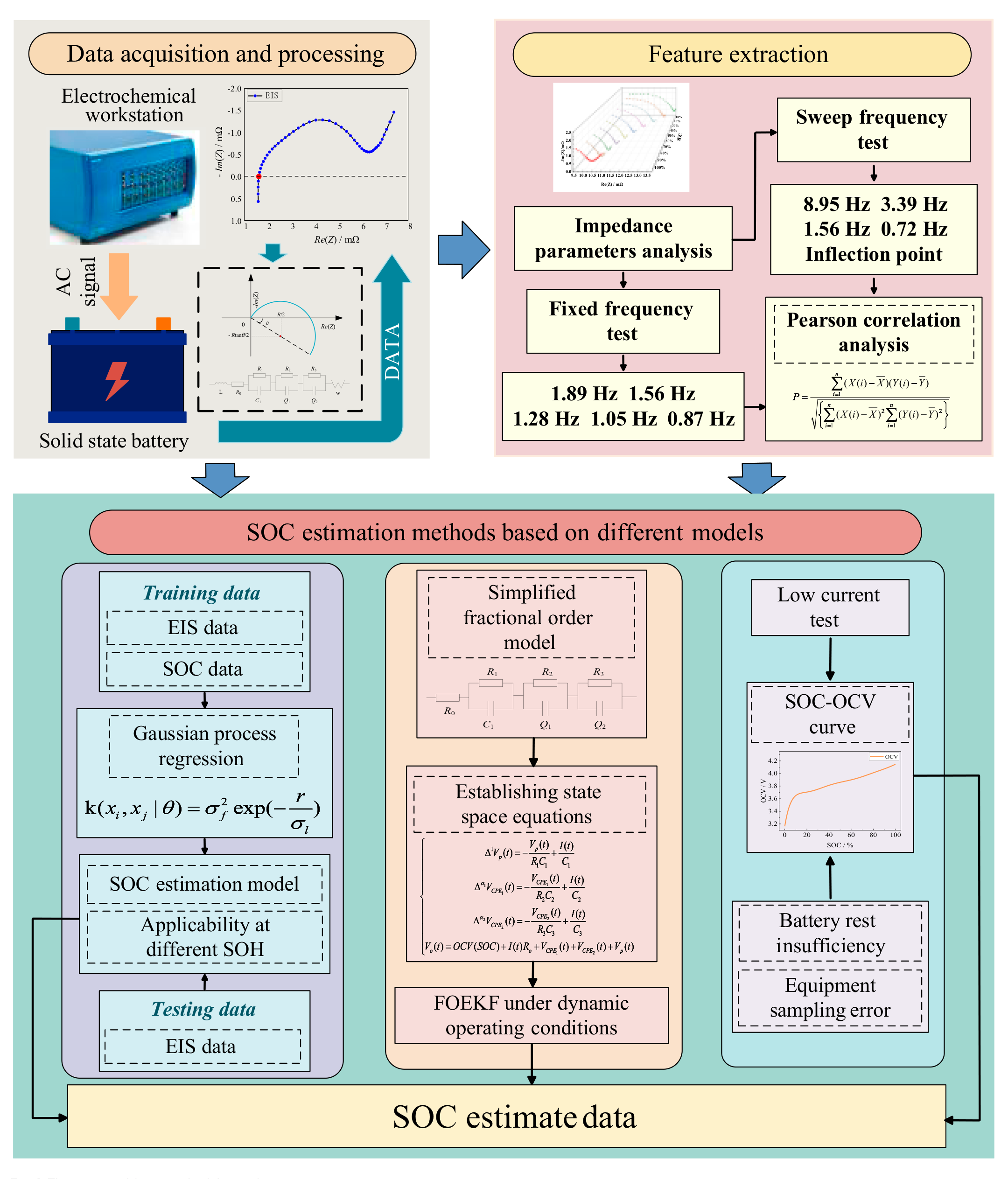
Fig. 1. The structural framework of the study.
GPR is a nonparametric model for regression analysis of data using a Gaussian process prior. It fits the corresponding Gaussian process through a finite amount of high-dimensional data to predict the value of the function under any random variable. In this paper, using health characteristics as input and battery capacity as output, the GPR exponential model is used for lithium-ion battery capacity estimation based on the MATLAB software tool with the kernel function shown in Eq. (10).
where is the standard deviation, r is the Euclidean distance, and is the scale parameter.
The KF algorithm is a method that uses input and output observations of a system to estimate its state. It is based on the theory of optimal estimation. While the original KF algorithm is only applicable to linear systems, the EKF algorithm can be used for nonlinear systems by linearizing them through the Taylor expansion. The FOEKF algorithm is based on the same concept as the EKF algorithm and combines it with the fractional-order model. This algorithm consists of a prediction step and an update step. The prediction step predicts the state variable at the next moment, while the update step updates the predicted value using the measurement data. The algorithm can be expressed as follows:
Determination of filtering initial conditions:
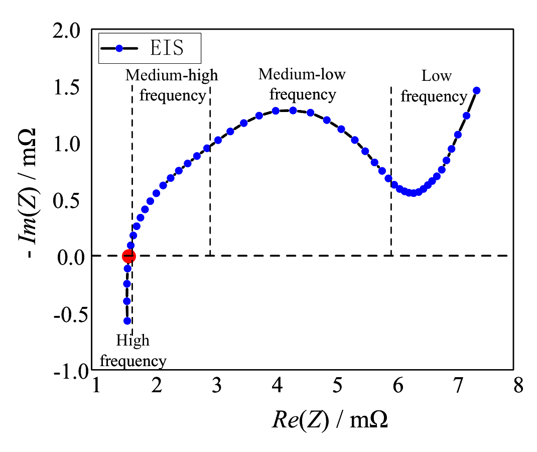
Fig. 2. Typical electrochemical impedance spectroscopy.
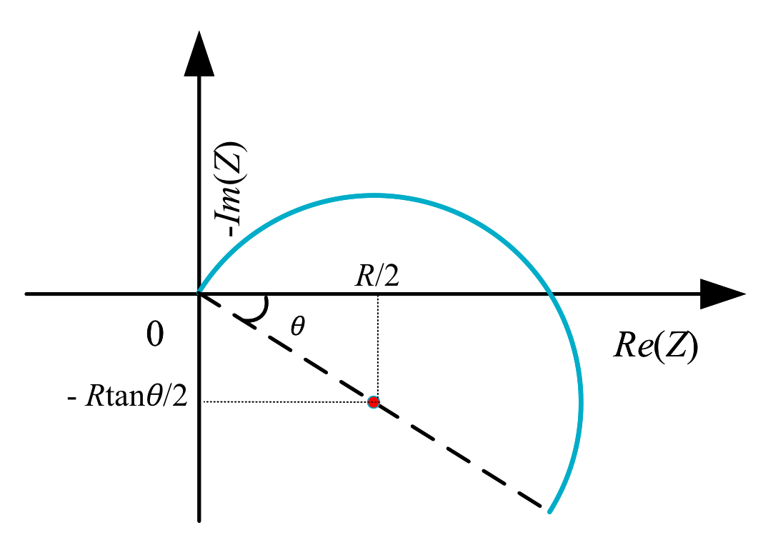
Fig. 3. Impedance diagram of parallel composite component RQ.
Prediction step (state estimate and error covariance ):
P_{k}^{-} = \big[\Delta T_{s}^{\boldsymbol{\alpha}} A + \mathrm{diag}(\boldsymbol{\alpha})\big] P_{k-1} \big[\Delta T_{s}^{\boldsymbol{\alpha}} A + \mathrm{diag}(\boldsymbol{\alpha})\big]^{\mathrm{T}} + \sum_{j=2}^{k} \boldsymbol{\gamma}_{j} P_{k-1} \boldsymbol{\gamma}_{j}^{\mathrm{T}} + Q_{k} \tag{13}
The gain matrix is updated:
Update step (state estimate and error covariance ):
where subscript k denotes the kth moment, superscript denotes the optimal estimate, right superscript denotes the predicted value, and is the voltage measurement.
For this experiment, 3 LiCoO solid-state batteries were chosen with varying degrees of aging. EIS tests were conducted at different SOCs. The battery related parameters are shown in Table 1.
The battery capacitance and impedance spectroscopy test platform has been set up and connected, as depicted in Fig. 4. This platform uses German Bio-Logic Company's VMP-300 to perform EIS tests, covering a frequency range of 10 Hz to 7 MHz. U.S. Arbin Instrumentation Company's charging-discharging equipment is utilized to achieve a current range of 10 A. To ensure that the battery is in a constant temperature environment during the experiments, a high- and low-temperature test chamber is used. This chamber can maintain a set temperature range of to °C with an accuracy of 0.5 °C. The experimental design is as follows:
Fully rested at 25 °C;
Charge the battery to 4.2 V at 1,460 mA, then constant voltage until the current is less than or equal to 365 mA;
Rest for 1 h;
Table 1. Solid-state battery parameter table
| Parameter | Value | Unit |
|---|---|---|
| Nominal capacity | 7,300 | mAh |
| Rated voltage | 3.75 | V |
| Charging cutoff voltage | 4.2 | V |
| Discharge cutoff voltage | 3.0 | V |
| Standard charge-discharge current | 1,460 | mA |
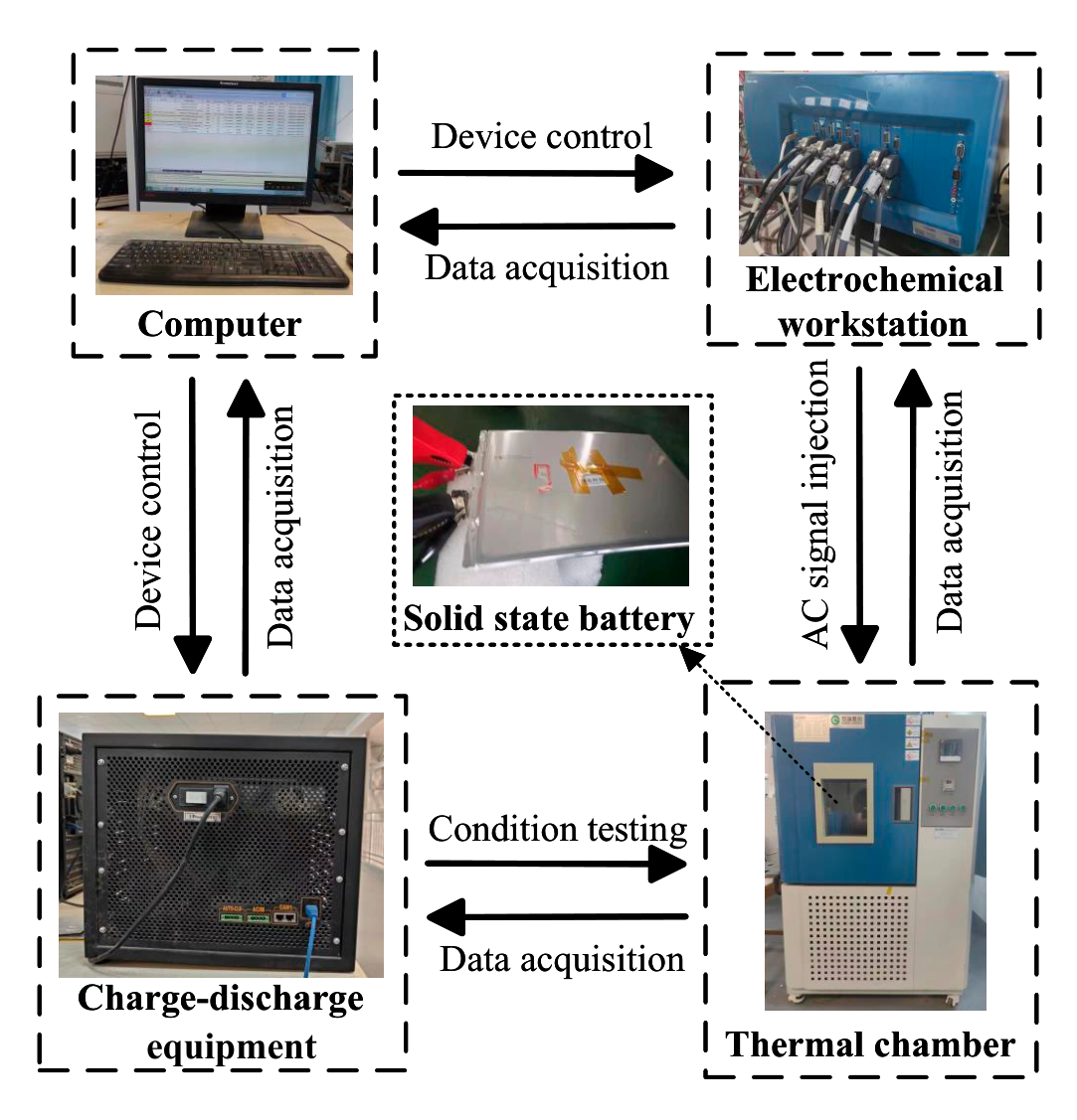
Fig. 4. The establishment of an experimental platform.
Discharges battery to 3.0 V at 1,460 mA;
Rest for 1 h;
Cycle ② to ⑤ 3 times, take the average of 3 times discharge capacity as the current battery capacity;
Charge the battery to 4.2 V at 1,460 mA, then constant voltage until the current is less than or equal to 365 mA;
EIS of the battery was performed at 100% SOC, and the battery was tested at 10 mV, with a frequency range from 100 kHz to 10 mHz, and 12 points were taken at each decibel frequency;
Discharge the battery 10% SOC at 1,460 mA and rest for 1 h;
Cycle 8 to 9 until battery voltage reaches 3.0 V;
Charge the battery to 4.2 V at 1,460 mA, then constant voltage until the current is less than or equal to 365 mA;
Rest for 1 h;
Cycle discharge the battery in DST (dynamic stress test) condition until the battery voltage reaches 3.0 V;
Rest for 1 h;
Charge the battery to 4.2 V at 1,460 mA, then constant voltage until the current is less than or equal to 365 mA;
Rest for 1 h;
Cycle discharge the battery in FUDS (full urban driving schedule) condition until the battery voltage reaches 3.0 V;
Rest for 1 h, end of experiment.
where ① to ⑥ are battery capacity calibration, ⑦ to ⑩ are the EIS test, and ⑪ to ⑱ are the working condition test.
The capacity of each battery was calibrated for standard working conditions. Battery #1 had a capacity of 6,753.73 mAh, battery #2 had a capacity of 7,014.56 mAh, and battery #3 had a capacity of 6,601.36 mAh. The EIS test results of the 3 batteries with different SOCs are shown in Fig. 5.
In Fig. 6, the variation of the last semicircle of the battery EIS with SOC is displayed. The battery EIS demonstrates regular changes as SOC decreases, with the middle-low frequency semicircle gradually spreading to the upper right. This correlation with battery SOC is strong.
where X and Y are the 2 variables for surrogate correlation, and are the average of the 2 variables for surrogate correlation, and n is the number of variables.
When , there is a weak correlation between the 2 variables; when , there is a moderate correlation between the 2 variables; when , there is a strong correlation between the 2 variables; and when , there is a perfect correlation between the 2 variables. If P is positive, there is a positive correlation; if P is negative, there is a negative correlation.
Fig. 8 analyzes the correlation between the above feature parameters and the battery SOC. As the battery SOC decreases, the battery impedance gradually increases, all 5 features show a negative correlation with the SOC, and the correlation coefficients are greater than 0.95, which shows a strong correlation, and it is suitable for estimating the battery SOC.
In this paper, batteries #1 and #2 are selected to train the SOC estimation model and #3 to validate the model. Five feature parameters are used as inputs for SOC estimation, and the Gaussian regression exponential model is selected for training based on the Regression Learner App of MATLAB. The estimation results of the model on the SOC of #3 battery after training are shown in Fig. 9, the maximum absolute error is not more than 1.5%, and the average absolute error is 0.564%, which can achieve the accurate estimation of SOC. However,
![Fig. 5. EIS test results for solid-state batteries (#1 - #3) with different SOCs. change of SOC, so it can be considered to select the appropriate frequency impedance and apply the online method to realize the EIS test and SOC estimation. Su et al. [ 28 ] utilize the step wave instead of a sine wave to achieve online acquisition of low-frequency EIS below 2 Hz without the aid of other equipment. In this paper, the impedance mode values at 5 frequencies of 1.89, 1.56, 1.28, 1.05, and 0.87 Hz are selected as the characteristic parameters. Their correlation coefficients with SOC are all above 0.95, showing strong correlation. They can be applied to estimate the SOC of the battery. The 5 frequency points are all under 2 Hz, and the stepped-wave method can be applied to obtain the EIS and achieve the SOC estimation by the online method. The 5 frequency points are all below 2 Hz, the stepped wave method can be applied online to obtain the EIS and realize the SOC estimation, the electrochemical workstation is applied to carry out the. A figure containing three Nyquist plots labeled #1, #2, and #3, each showing electrochemical impedance spectroscopy (EIS) results for a solid-state battery. Each panel plots the negative imaginary part of impedance (-Im(Z)) in mΩ versus the real part (Re(Z)) in mΩ, with multiple data series corresponding to different states of charge (SOC) ranging from 10% to 100%, identified in a legend with distinct markers. Each panel includes a zoomed inset highlighting a region of interest indicated by an arrow, showing the detailed behavior of the curves where they cluster.](/debrief/space-soc-estimation/images/figure_05.png)
Fig. 5. EIS test results for solid-state batteries (#1 - #3) with different SOCs.
the frequency corresponding to the low-frequency inflection point of the EIS gradually decreases with the decrease of SOC, and to accurately determine the inflection point, it is necessary to carry out a frequency sweep test of the EIS of the middle and low-frequency bands, and then to determine the inflection point with the geometric characteristics. Taking this battery as an example, the EIS band shown in Fig. 6 is [10.866 Hz, 0.103 Hz], and 6 points are taken for each 10-fold frequency, which is tested by the electrochemical workstation in about 122 s, taking a relatively long time, and does not take advantage of the rapid estimation of the SOC of solid-state batteries for practical applications.
Observing the semicircle in Fig. 6, it can be seen that the whole semicircle shows an obvious change rule with the fixed-frequency test in the laboratory, and the data acquisition time is about 25 s, which is fast.
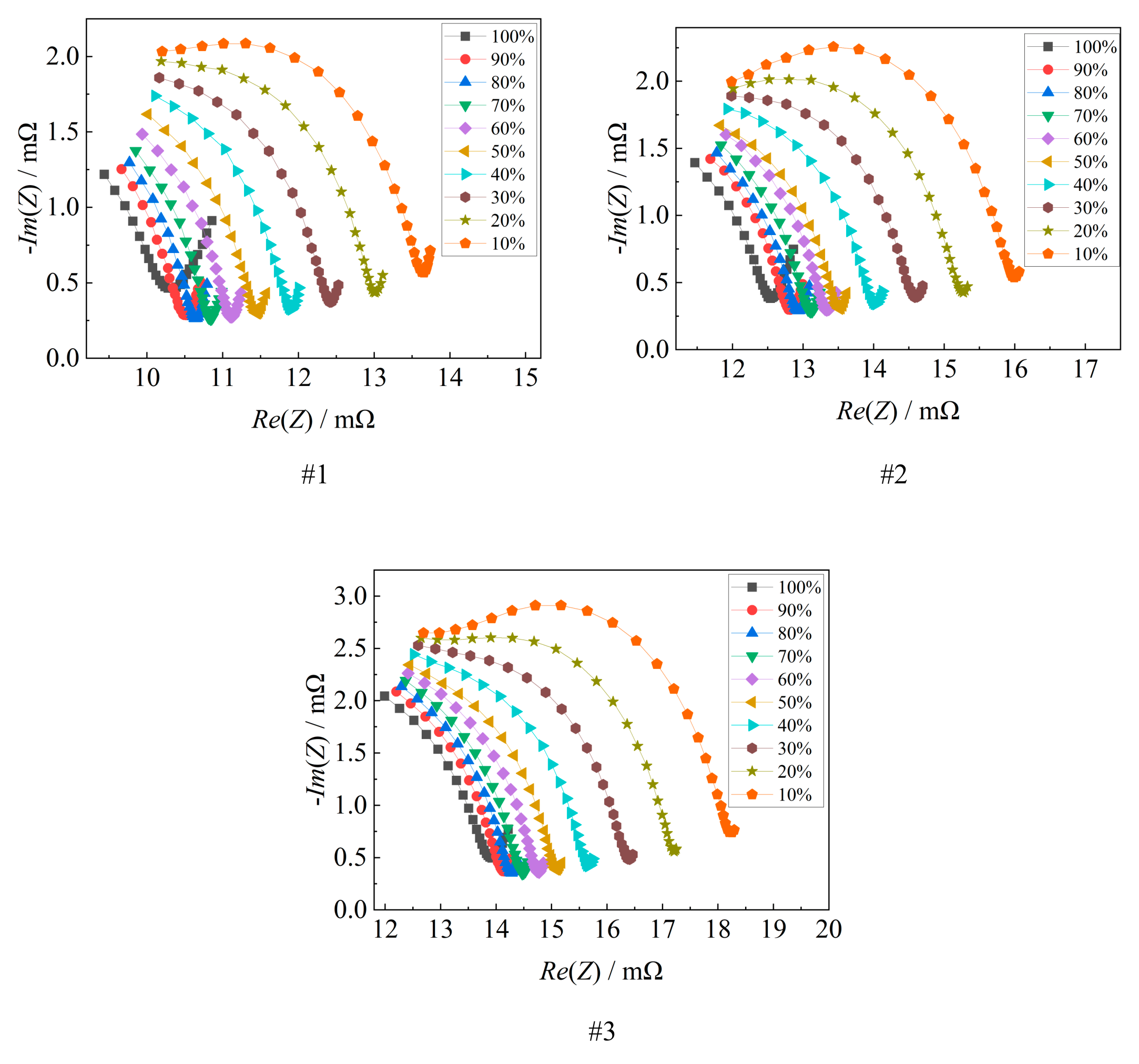
Fig. 6. Medium-low-frequency semicircle of solid-state battery (#1 - #3) with different SOC.
The above Gaussian regression exponential model is applied to train the model and estimate the SOC of battery #3, and the estimation results are shown in Fig. 10. The characteristic parameters show good estimation results, with the maximum absolute error of 1.5989% and the average absolute error of 0.2998%, which achieves the fast estimation of SOC taking into account the accuracy.
Since the SOHs of the 3 batteries used are different, the 3 batteries are used as the training set and validation set to build the SOC estimation model with the abovementioned fixed-frequency extracted features as an example, and to validate the applicability of the method to build the model under different SOHs. The grouping is shown in Fig. 11.
The EIS of this solid-state cell in different SOC states is shown in Fig. 5, and as the SOC decreases, the last semicircle in the impedance spectrum in the low frequency gradually comes to the forefront, and the distribution of relaxation time (DRT)
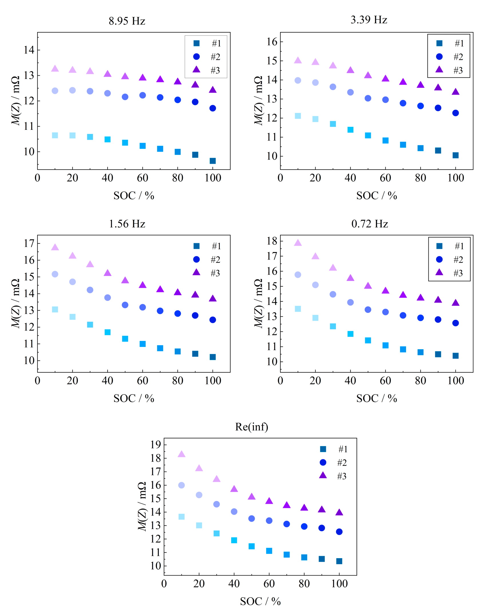
Fig. 7. The trend of characteristic parameters changing with SOC.
analysis of the EIS of the solid-state battery is carried out by using the tool from [31]. As shown in Fig. 12, this solid-state cell is decomposed into 5 relaxation time peaks. The semicircle above the real axis of the EIS is broken up into 3 parts, which adds an unknown electrochemical process to the solid-state cell over the lithium-ion cell. As shown in Fig. 5B, there are 3 semicircles above the real axis of the EIS for cell #2. Based on the specificity of the EIS of this solid-state battery, this paper proposes to fit the EIS through the third-order RC, taking into account the offset caused by the “dispersion effect”, and the 2 RCs are replaced by RQ. The EIS is fitted through the fractional-order model shown in Fig. 13. The impedance expression is shown in Eq. (18). The impedance spectral fitting software ZSimpWin is used to verify the fitting of the fractional-order model, as shown in Fig. 14, which is verified to be able to characterize the impedance spectral information under different SOC states.
To verify the fitting effect of the model, the fitting error is defined as shown in Eq. (19), and the error of fractional-order model fitting EIS of each SOC point of 3 batteries is calculated. The results are shown in Table 3. The model can better fit the EIS of the solid-state battery.
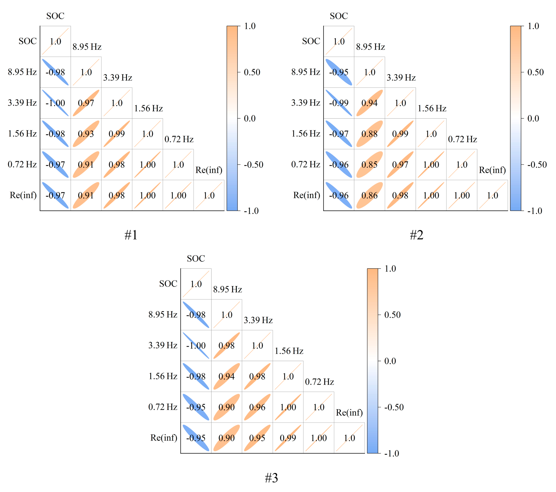
Fig. 8. The correlation between feature parameters and SOC.
where , denotes the impedance real and imaginary part fitted values, and Re, Im denotes the impedance real and imaginary part measured values.
To simplify the parameters and reduce the computational effort of the fractional-order extended KF algorithm, the inductance of the high-frequency inductive part and the Warburg impedance of the low-frequency diffusion process are neglected. Therefore, the fractional-order equivalent circuit model of the solid-state battery consists of an integer-order RC network, 2 fractional-order RQ networks, and the ohmic internal resistance and the OCV. The expression for the terminal voltage of the fractional-order equivalent circuit model is:
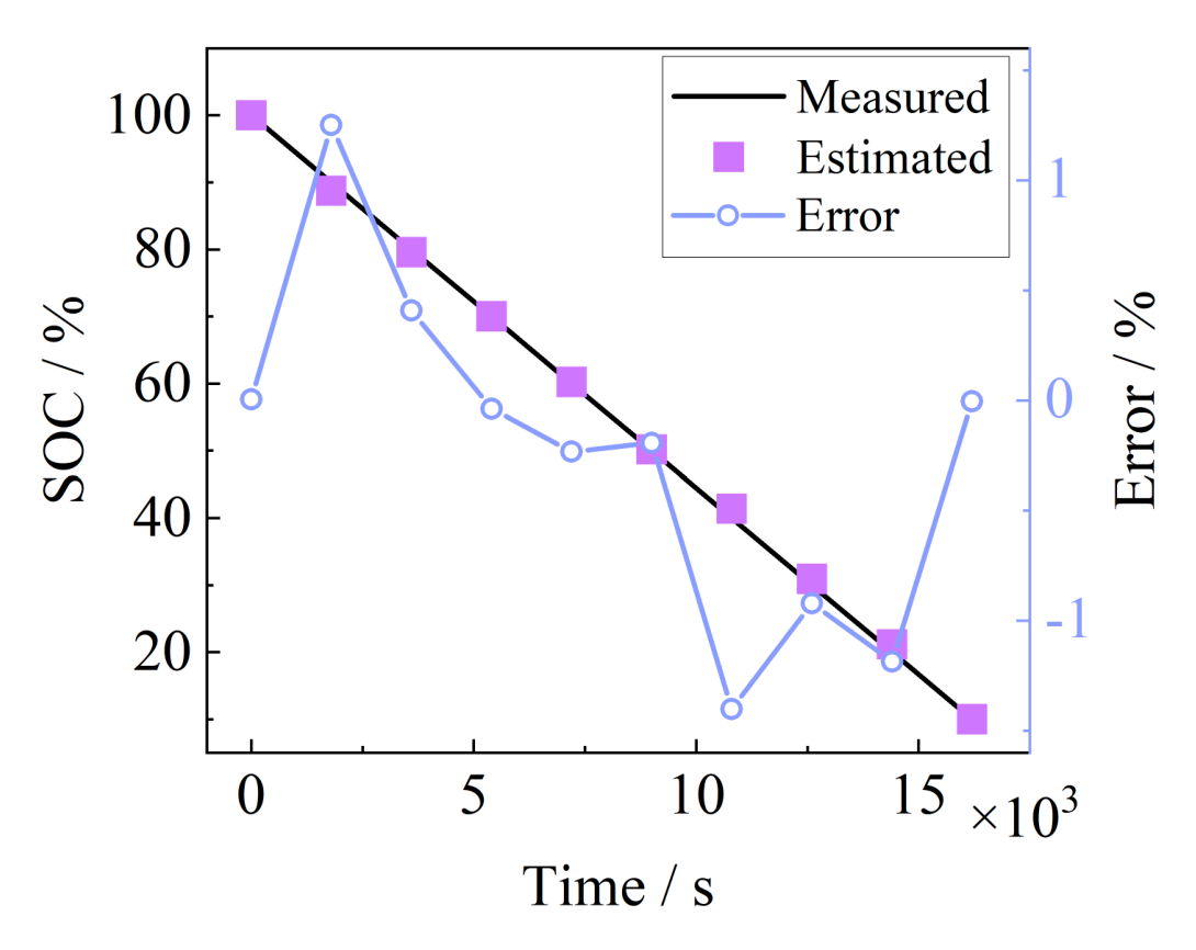
Fig. 9. SOC estimation results.
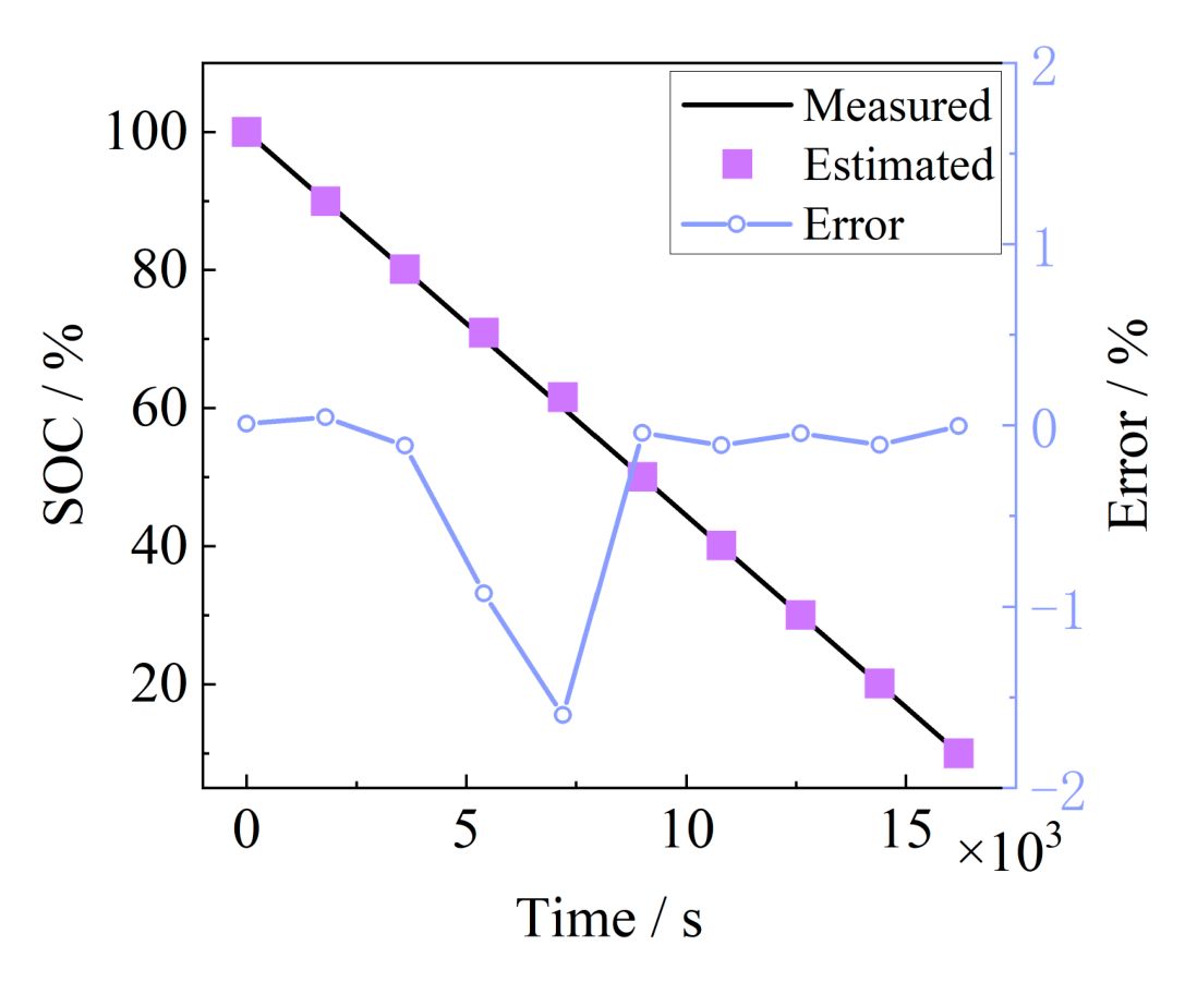
Fig. 10. Fixed-frequency feature SOC estimation results.
| #1 | #2 | #3 |
|---|---|---|
| Training | Training | Testing |
| Training | Testing | Training |
| Testing | Training | Training |
Fig. 11. Different SOH batteries grouped as training sets.
Table 2. Results of training models with different SOH batteries
| Group | MaxAE/% | MAE/% |
|---|---|---|
| Group 1 | 1.5989 | 0.2998 |
| Group 2 | 5.0965 | 1.5422 |
| Group 3 | 2.4604 | 0.9927 |
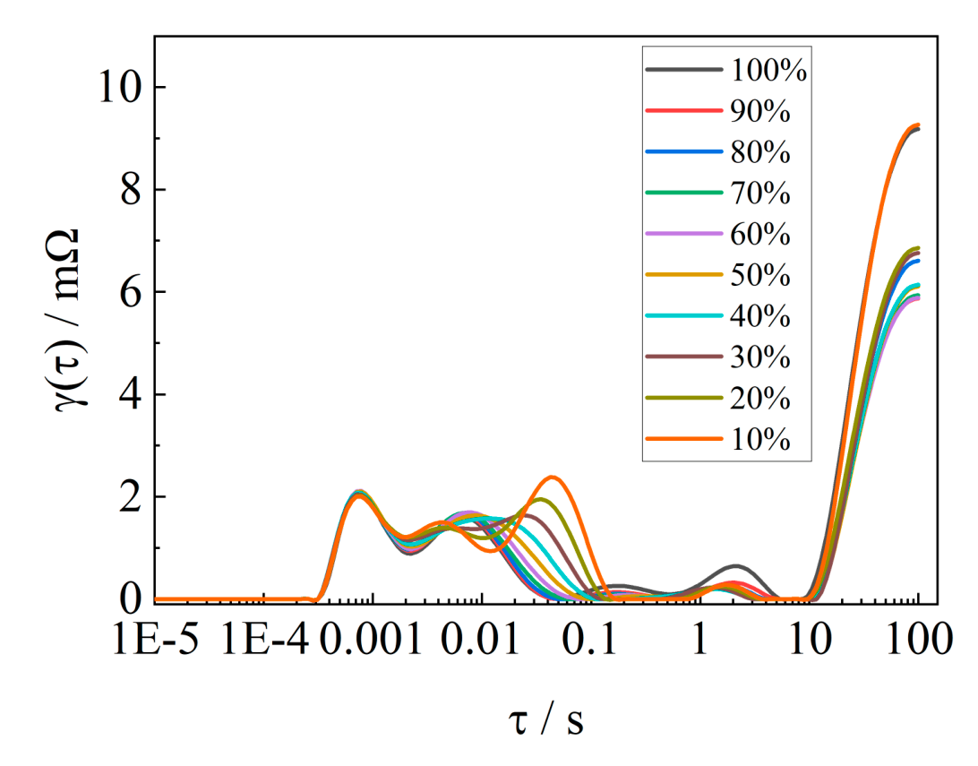
Fig. 12. DRT analysis of different batteries.
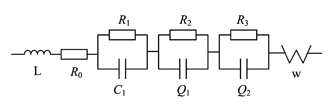
Fig. 13. Fractional-order model.
where and are the orders; , , and are the polarization voltages of the integer order and fractional-order networks; I is the current through the battery, which is taken to be positive in the direction of charging; and OCV is the OCV, which is a polynomial function of the polynomial curve about the SOC, with the specific expression of Eq. (21), which is only affected by the ambient temperature and battery aging.
where to denote the polynomial fitting coefficients. In addition, the amount of change in cell SOC at moment is:
where Q is the actual maximum available capacity of the solid-state battery. Taking the state variable , the state transfer matrix is obtained from Eqs. (21) and (22), and the observation matrix , which leads to and , with , and the fractional-order differential operator . At this point, Eq. (20) can be written in the following form:
Combining Eq. (7), then Eq. (24) holds. Where
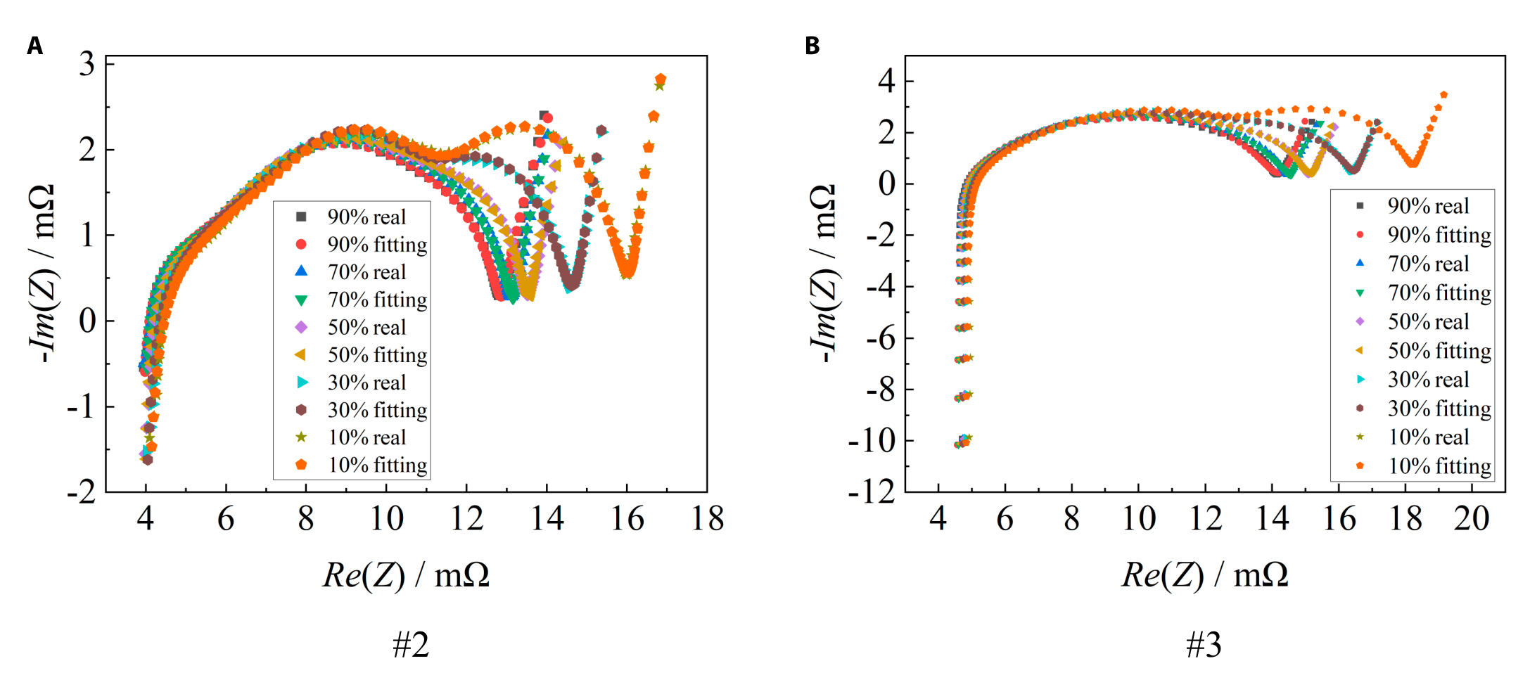
Fig. 14. Fractional-order model fitting effect for #2 and #3.
Table 3. Fractional-order model fitting error
| Battery SOC | #1 | #2 | #3 | |||
|---|---|---|---|---|---|---|
| Err/mΩ | Err/% | Err/mΩ | Err/% | Err/mΩ | Err/% | |
| 100% | 0.070 | 0.768 | 0.043 | 0.445 | 0.055 | 0.577 |
| 90% | 0.040 | 0.441 | 0.022 | 0.283 | 0.072 | 0.763 |
| 80% | 0.058 | 0.607 | 0.058 | 0.570 | 0.065 | 0.648 |
| 70% | 0.052 | 0.535 | 0.025 | 0.294 | 0.060 | 0.668 |
| 60% | 0.098 | 1.020 | 0.062 | 0.587 | 0.059 | 0.662 |
| 50% | 0.098 | 0.998 | 0.024 | 0.280 | 0.028 | 0.334 |
| 40% | 0.070 | 0.708 | 0.088 | 0.759 | 0.055 | 0.606 |
| 30% | 0.089 | 0.862 | 0.038 | 0.515 | 0.050 | 0.559 |
| 20% | 0.065 | 0.609 | 0.116 | 1.274 | 0.057 | 0.576 |
| 10% | 0.059 | 0.531 | 0.043 | 0.535 | 0.030 | 0.368 |
Ultimately, the general form of the discrete expression of the state space equation for the fractional-order model of the solid-state battery is obtained as:
where is the process noise with mean 0 and covariance , is the measurement noise with mean 0 and covariance , and and are uncorrelated.
The voltage simulation accuracy of the above fractional-order model is verified through different working conditions, and the simulation results are shown in Fig. 15. The RMSE (root mean square error) of the voltage simulation is 8 mV for the DST condition, and the RMSE of the voltage simulation is 7.3 mV for the FUDS condition, which shows that the above fractional-order model can simulate the battery voltage well and can be used for the SOC estimation.
The above EKF algorithm based on the fractional-order model performs the SOC estimation, and the accuracy is verified using DST and FUDS working conditions. First, the initial value is set to 50% SOC, and the SOC estimation results of different working conditions are shown in Fig. 16. The DST condition converges to an error of no more than 5% after 58 s and to an error of no more than 2% after 126 s, the converged estimation results have a slight deviation of more than 2% at around 45% SOC, and the rest of the estimation results have errors of less than 1%. The FUDS condition converges to an error of no more than 5% after 53 s and to an error of no more than 2% after 109 s, and the converged estimation results are good with an error of less than 1%.
Different initial values are set under FUDS conditions to verify the convergence speed and estimation accuracy of FOEKF. The initial SOC is set to be 0%, 30%, 60%, and 90%, respectively. The estimation results are shown in Fig. 17, and the convergence time for different initial values is shown in Table 4. The FOEKF algorithm can be effectively corrected when the initial value of the battery is unknown, but the convergence speed is affected by the deviation of the initial value,
and the larger the deviation of the initial value, the slower the convergence speed.
Currently, the SOC estimation of electric vehicles mostly uses the ampere-time integration method, and the determination of the initial value becomes the main factor affecting its accuracy. The acquisition of the initial value can be calculated based on the SOC-OCV curve lookup table, while the acquisition of OCV requires the battery to be stationary for a long time. Therefore, the OCV can be accurately obtained only when the vehicle is parked and restarted for longer. When the quiescence
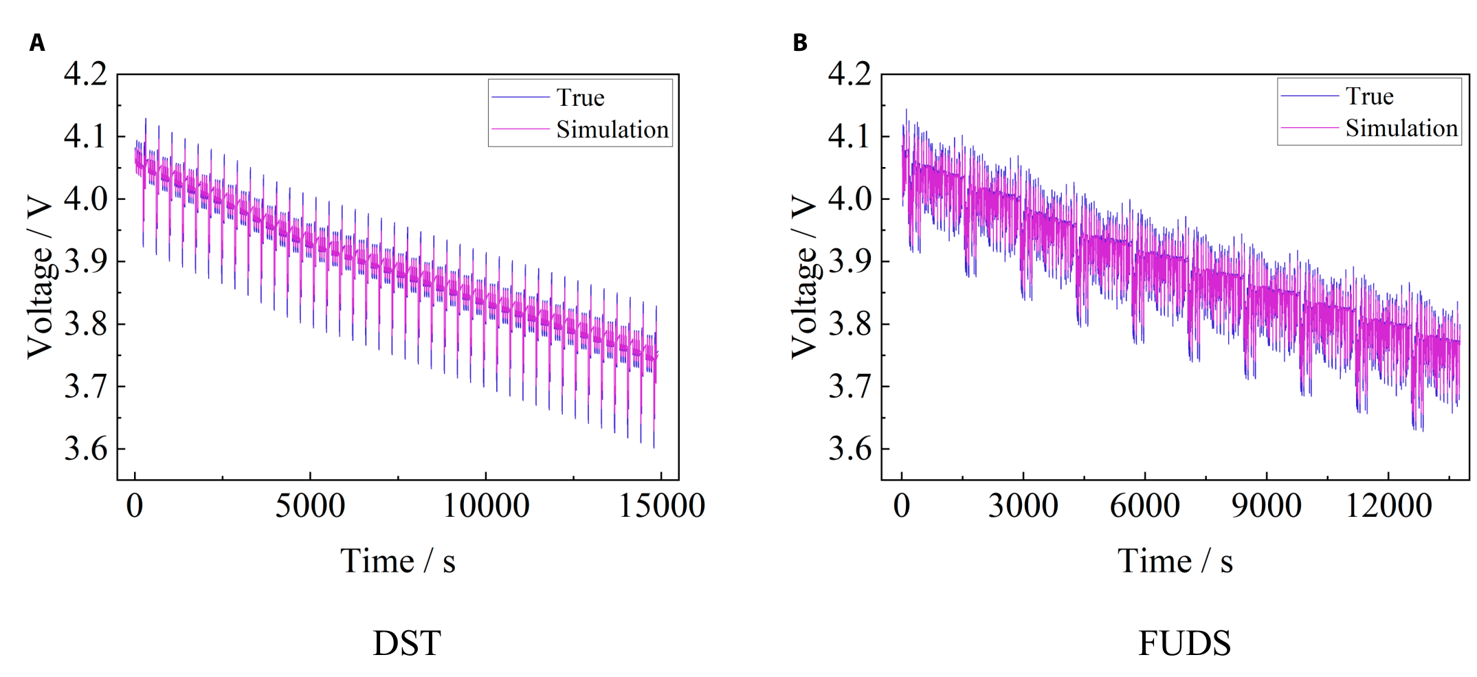
Fig. 15. Voltage simulation results under different working conditions — DST (A) and FUDS (B).
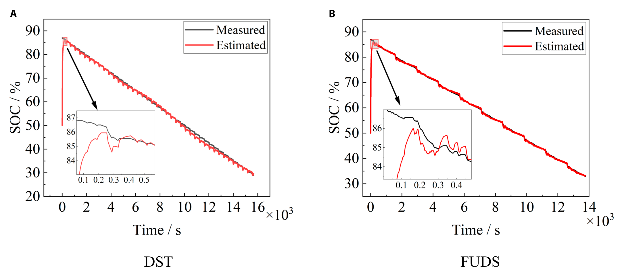
Fig. 16. Fractional EKF estimation of SOC under different operating conditions — DST (A) and FUDS (B).
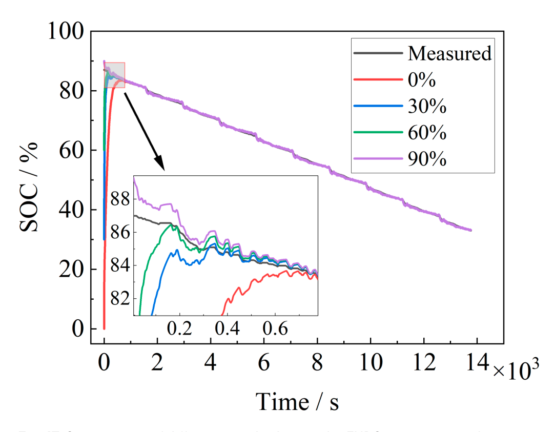
Fig. 17. Convergence of different initial values under FUDS operating conditions.
Table 4. Initial value convergence under FUDS working condition
| Initial value | Less than 5% error in time/s | Less than 2% error in time/s |
|---|---|---|
| 0% | 329 | 446 |
| 30% | 93 | 157 |
| 60% | 38 | 81 |
| 90% | Initial error less than 5% | 12 |
Table 5. Comparison of SOC estimation methods for solid-state battery
| Method | Advantage | Disadvantage |
|---|---|---|
| FOEKF | Convergence of initial values | Long convergence time, greatly influenced by initial values. The model needs to obtain complete EIS data. |
| SOC-OCV curve | The results are accurate and do not require algorithms | The battery needs to be left standing for a long time. Only applicable to single-point estimation. |
| EIS parameters | Accurate estimation and short-time consumption | Different frequency impedance tests need to be conducted on the battery. |
is not sufficient or the sampling error precision of the equipment is limited, the OCV will not be accurately obtained, which also leads to the introduction of SOC estimation error, especially when there is a voltage plateau in the battery OCV, and the error will be greatly increased. The SOC-OCV curve of this solid-state battery is shown in Fig. 18, and the SOC of the current battery can be obtained by obtaining the battery OCV and using the mapping relationship between OCV and SOC of this curve.
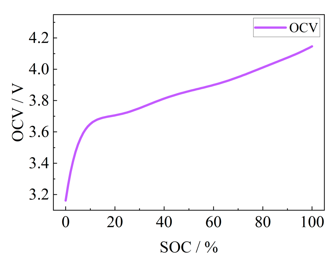
Fig. 18 SOC-OCV curve.
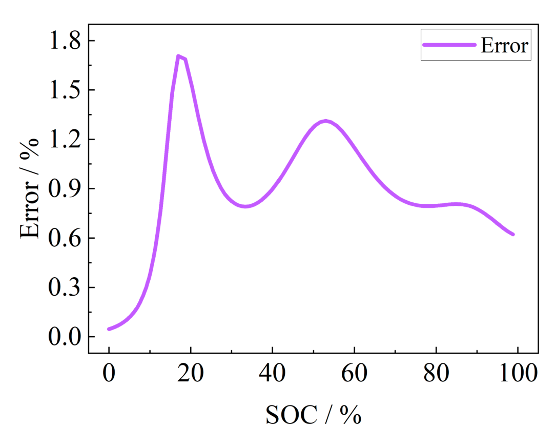
Fig. 19. Absolute error generated by sampling under different SOC.
All of the above methods can achieve a more accurate estimation of the SOC of solid-state batteries, but there are certain advantages, disadvantages, and applicability of each method, as shown in Table 5.
Among the above 3 methods, the EIS estimation method needs to test the EIS of the battery, even if the fixed-frequency points below 2 Hz can be measured without other equipment, but it takes 25 s to obtain the parameters. The estimation process mainly consists of importing data into the model and outputting the results, and the estimation process time can be ignored, which can be used for the initial SOC calibration and is almost unaffected by the battery SOH, as long as a good model is trained. The FOEKF method is mainly for online real-time applications, and online estimation can be realized as long as the model is built, but its model needs to be updated according to the change of the SOH of the battery. The SOC-OCV method can be mainly used for the calibration of the initial SOC, which can be almost instantly accomplished by only measuring the battery voltage, but it also needs to update the curve with the change of the SOH of the battery. Therefore, each of the 3 methods has its advantages and disadvantages. The SOC-OCV method and the EIS method can be used for initial SOC calibration. In terms of computational cost, the SOC-OCV method has a lower computational cost, but it depends on the timely updating of the curves with the change of SOH, while the EIS method is able to avoid this problem.
The results show that establishing an estimation model based on EIS extracted features can balance accuracy and speed. If the online implementation method of EIS is combined with the extraction of battery fixed-frequency impedance modulus as a feature parameter, it is expected to achieve the accurate estimation of online SOC for the full cycle of solid-state battery operation.
This paper addresses the existing research gap in modeling and parameter estimation for solid-state batteries. It presents a novel approach by extracting impedance parameters at various frequencies using EIS testing, leading to the development of a solid-state battery SOC estimation model. This model enables fast and precise SOC estimation for solid-state batteries. Additionally, the article performs a thorough analysis of 2 other methods, namely, the FOEKF and the SOC-OCV table lookup approach. By evaluating the strengths and weaknesses of these methods, the article provides valuable insights into their suitability for SOC estimation in the context of solid-state batteries.
Considering the 3 semicircular frequency bands of solid-state battery EIS, the RQ process is added to establish a fractional-order model applicable to solid-state batteries, and the SOC estimation model is established by combining the FOEKF algorithm. The estimation accuracy is verified by DST and FUDS dynamic working conditions, and the convergence time
and estimation accuracy of different initial values are analyzed. Then, the estimation error of the SOC-OCV method is analyzed by the resting insufficiency and sampling error.
Funding: This work was supported by the National Natural Science Foundation of China (grant no. 52177206) and Beijing Nova Program (grant no. 20220484153).
Author contributions: J.P. performed the numerical experiments. X.Z. and J.P. analyzed the data. All the authors contributed to the writing and revising of the manuscript.
Competing interests: The authors declare that they have no competing interests.
The data are available from the authors upon a reasonable request.
Search is free. Join the waitlist to open papers and ask your own questions across the full catalog.
Ask in a sentence, the way you'd ask a colleague. Debrief matches on meaning — no keyword guessing or filter-stacking.
Ask any paper in plain language. Each answer arrives with a citation to the exact section and page it came from.
Every result is tagged peer-reviewed, preprint, or manuscript — so you weigh the evidence, not just the words.
Tap a citation and it jumps you to that exact paragraph in the full paper — never bounced out to a PDF.
Early Access
Free during early access. No credit card. No commitments.